How to do ecological research

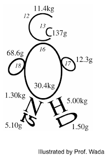
Stable Isotope  Isotope is defined as elements with same atomic number (= same number of protons) and different neutron number. Therefore, isotopes of an elements have different mass. For example,  12 C,    13 C   and  14 C  are all carbon isotopes and  13 C  and  14 C  are heavier isotopes than  12 C   Stable isotopes are isotopes which is stable without radioactive decay.  14 N  is a radioactive isotope emitting radioactive radiation, eventually collapsing into  14 N  while  13 C  is a stable isotope which remain stable in nature. Usually, heavier stable isotopes exist in very little amount in nature. In a person of 50 kg,  13 C  weighs only 137g while  12 C  does 11.4 kg. For nitrogen, 15N weighs only 5.1 g while 14N does 1.3 kg.   Fig. 1. An 'isotope man' illustrated by Prof. Eitaro Wada.   http://www.lowtem.hokudai.ac.jp/isophysiol/pg39.html Most studied isotopes are as below:      Hydrogen:  1 H ,  2 H ,  3 H  (radioactive)      Carbon:  12 C ,  13 C ,  14 C  (radioactive

Since principal component analysis (PCA) is the most basic and commonly used dimensionality reduction method, I would like to explain some basis to understand PCA used in ecological research. As analysis of variance (ANOVA) can decompose total variance into variances explained by factors and error, PCA attempts to find new axes to explain the most variability of your multivariate data. Let us assume that your data has 100 variables for each observation.  Say one forest site has 100 species abundances or one chromatogram has 100 peak areas. If you want to compare your observations and to find ecological patterns, you need to plot 100-d space with 100 axes, which is only possible in mathematical world.  In mathematics, you can produce N-dimensional hypervolume such as Hutchison' niche concept (Hutchinson 1957). However, it is hard to visualize 100-d space.   If we can reduce 100-d data into 2 or 3-d data, we can visualize your data in 2-d or 3-d space.  That is dimensionality reduc

Ecological research usually deals with large numbers of variables such as species compositions with many species or biological responses with many environmental factors.  To recognize ecological patterns, we first look correlations and regressions on 2-d or 3-d space. What if your variables are so many, say more than a hundreds? There is no way to plot 100 d space for pattern recognition.  Biotic community can easily have more than hundred species and when you want to compare species compositions of 30 plots in your study, you need something to summarize species composition to compare your plots.  In those cases, you can use dimensionality reduction such as principal component analysis (PCA), non-metric multidimensional scaling (NMS), corresponding analysis (CA), detrended corresponding analysis (DCA), and canonical corresponding analysis (CCA), etc. Fig. 1  An example showing  the c oncept of dimensionality reduction. Species composition data (left) of seed banks at three differe

Analysis of Variance (ANOVA) is one of the most commonly applied statistical analysis in ecological research.  Many scientists in ecology area use ANOVA to test whether averages of more than two groups are same or not.  It is an extension of t-test which tests whether averages of two groups are same or not.  For example, let us assume that we are testing averages of three different group.  If averages of all three groups are not so different, the variance among groups (variance for three average values) would be very small. However, you also consider variances within group (variance for each data from their group average). Fig. 1 Concept for analysis of variance (ANOVA) showing total variance is sum of variance for among groups and variance for within group.   ©S Park If the among group variance is large enough compared to within group variance, we may say that averages of these three groups are significantly different.  To test the null hypothesis ("Three group averages ar